TD Learning model simulation

Through Temporal Difference (TD) learning, an agent learns from future rewards and back-propagates prediction errors by updating value estimates. Basically, the agent is continually updating beliefs about future rewards as it approaches the future. It is the core concept of model-free reinforcement learning.

Variables

Conditioned stimulus: $ u \in \{ 0,1 \} $ .

Unconditioned stimulus: $ r\in \{ 0,1 \} $ .

The linear filter used to build convolutional kernel: $ w\in \mathbb{R} $ .

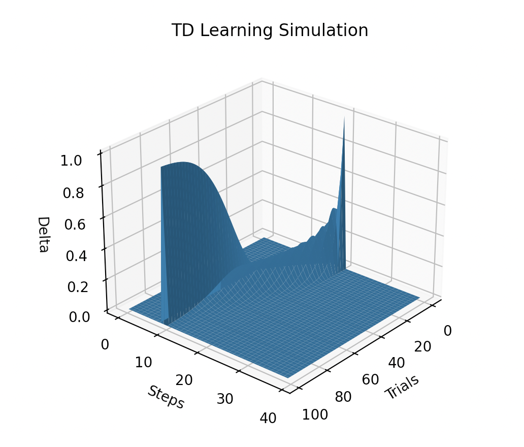
As learning progresses, the prediction error upon receiving a reward will gradually decrease to zero. This means there will be less and eventually no surprise when obtaining the reward.

The prediction error will propagate back to the cue onset time. Once the animal hears the cue, the prediction error (surprise) occurs.

Learning process

Similar to the Rescorla-Wagner rule - designed to minimise $\frac{1}{2} \delta^2$ , adjust value with the TD learning rule:

$$V_t = \sum_{\tau=0}^t w(\tau)u(t-\tau)$$

$$V_{t+1} = \sum_{\tau=0}^{t+1} w(\tau)u(t+1-\tau)$$

$$ \delta_t = r_t + V_{t+1} - V_t $$

$$ w(\tau) \leftarrow w(\tau) + \alpha\delta_tu(t-\tau)$$

$\alpha$ is the learning rate. $\delta_t$ is the prediction error at time $t$ .

A demo

Assume that the cue onset at time 2( $u_2=1$ and $u_{others}=0$ ), and reward onset at time 5( $r_5=1$ and $r_{others}=0$ ). Set learning rate $\alpha$ as $0.5$ .

In the first trial, update prediction error $\delta_t$ at time $t=5$ , when the reward is obtained.

$$\delta_5 = r_5 + V_6 - V_5 = 1+0-0=1$$

Then update parameter

$$w_3 \leftarrow w_3 + \alpha\delta_5 u_2 = 0+0.5\times1\times1=0.5$$

which is equvalent to update value

$$V_5 \leftarrow V_5 + \alpha\delta_5 = 0+0.5\times1=0.5$$

Since $$V_5 = w_0u_5 + w_1u_4 + w_2u_3 + w_3u_2 + w_4u_1 + w_5u_0 = w_3 u_2 $$

$$\frac{dV_5}{dw_3} = u_2$$

In the second trial,

at time $t=4$ , update

$$\delta_4 = r_4 + V_5 - V_4 = 0+0.5-0=0.5$$

$$w_2 \leftarrow w_2 + \alpha\delta_4 u_2 = 0+0.5\times0.5\times1 = 0.25$$

at time $t=5$ , update

$$\delta_5 = r_5 + V_6 - V_5 = 1+0-0.5=0.5$$

$$w_3 \leftarrow w_3 + \alpha\delta_5 u_2 = 0.5+0.5\times0.5\times1 = 0.75$$

In the third trial, update $w_3, w_2, w_1$ . In the fourth and following trials, update $w_3, w_2, w_1, w_0$ , until prediction error converges to zero.

Simulation

# TD Learning model

import matplotlib.pyplot as plt
import numpy as np


def td_learn(lr=0.2, trials_n=100, steps_n=40, cs=10, us=20):
    """TD Learning

    Args:
        lr (float): learning rate. Defaults to 0.2.
        trials_n (int): number of trials. Defaults to 100.
        steps_n (int): number of steps per trial. Defaults to 40.
        cs (int): conditioned stimulus onset. Defaults to 10.
        us (int): unconditioned stimulus onset step. Defaults to 20.
    """
    # cue(unconditioned stimulus) onset at step cs
    u = np.zeros(steps_n)
    u[cs] = 1

    # reward(conditioned stimulus) onset at step us
    r = np.zeros(steps_n)
    r[us] = 1

    # w is the linear filter for convolutionary kernel
    w = np.zeros((steps_n, trials_n))

    # init to store v and delta
    v = np.zeros((steps_n, trials_n))
    delta = np.zeros((steps_n, trials_n))

    # learning session
    for t_i in range(trials_n - 1):
        for s_i in range(steps_n - 1):
            # update v(values) by linear filter w
            v[s_i, t_i] = w[:s_i+1, t_i] @ u[s_i::-1]
            v[s_i+1, t_i] = w[:s_i+1+1, t_i] @ u[s_i+1::-1]

            # prediction error delta
            delta[s_i, t_i] = r[s_i] + v[s_i+1, t_i] - v[s_i, t_i]

            # update parameters
            # v[s_i, t_i] += lr * delta[s_i, t_i]
            w[:s_i+1, t_i] += lr * delta[s_i, t_i] * u[s_i::-1]

        # v[:, t_i+1] = v[:, t_i]
        # save w for the next trial
        w[:, t_i+1] = w[:, t_i]

    return delta, w, v


def plot(trials_n, steps_n, num):

    x = np.arange(0, trials_n)
    y = np.arange(0, steps_n)

    X, Y = np.meshgrid(x, y)
    Z = num

    fig = plt.figure()
    ax = fig.add_subplot(111, projection='3d')
    ax.plot_surface(X, Y, Z)

    ax.set_xlabel('Trials')
    ax.set_ylabel('Steps')
    ax.set_zlabel('Delta')

    ax.set_title('TD Learning Simulation')

    plt.show()


lr = 0.2
trials_n = 100
steps_n = 40

delta, w, v = td_learn(lr, trials_n, steps_n, cs=10, us=20)
# print(delta)
plot(trials_n, steps_n, delta)

d019-rl-05-img1

Reference