Rescorla–Wagner model simulation

The Rescorla-Wagner model captures key aspects of classical conditioning(Pavlovian experiment). It is based on a simple linear equation that predicts the reward associated with a stimulus.

Variables

Conditioned stimulus: $ x \in \{ 0,1 \} $.

Unconditioned stimulus: $ r\in \{ 0,1 \} $.

Associative strength between $x$ and $r$: $ w\in \mathbb{R} $.

e.g. by hearing a tone $x$, how likely $w$ the animal would think of cheese $r$.

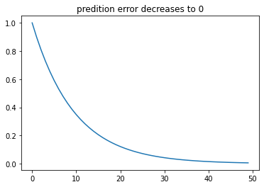
Prediction error: $ \delta = r-wx $

With learning, the prediction error will gradually approach zero, meaning there will be less and eventually no more prediction error or, say, no more surprise.

Learning process

How does the associative strength change? i.e. How does animal learn that the tone and cheese are associated?

Following the Rescorla-Wagner rule - designed to minimise $\frac{1}{2} \delta^2$, associative streghth $w$ is updated by linearly adding a prediction error, adjusted by the learning rate $\alpha$, i.e. how fast the animal learn.

$$ w \leftarrow w + \alpha(r - wx)x$$

If x is always 1(i.e. there is always cheese following a tone), simplify the above equation as

$$ w \leftarrow w + \alpha(r - w)$$

PS. The learning process designed by the R-W rule is the same as stochastic gradient ascent(SGA).

The gradient of $\frac{1}{2} \delta^2$ is

$$ grad = \frac{d}{dw} \frac{1}{2} \delta^2 = \frac{d}{dw} \frac{1}{2} (r-wx)^2 = (r-wx)x$$

Update $w$ by

$$ w \leftarrow w + \alpha \times grad $$

which is exactly

$$ w \leftarrow w + \alpha(r - wx)x $$

Simulation

# R-W Model

import numpy as np
import matplotlib.pyplot as plt

trial_ind = np.array(range(50))

x_lst = np.full(len(trial_ind), 1)
r_lst = np.full(len(trial_ind), 1)
w_lst = []
delta_lst = []

# init
w_lst.append(0)

lr = 0.1

for i in range(len(trial_ind)):
    delta = r_lst[i] - w_lst[i] * x_lst[i]
    w = w_lst[i] + lr * delta
    delta_lst.append(delta)
    w_lst.append(w)

# remove init w
w_lst.pop(0)

# plot
plt.title("predition error decreases to 0")
plt.plot(trial_ind, delta_lst)

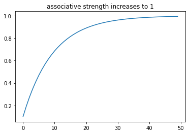
plt.title("associative strength increases to 1")
plt.plot(trial_ind, w_lst)

Reference

Dayan, Peter, and Laurence F. Abbott. Theoretical neuroscience: computational and mathematical modeling of neural systems. MIT press, 2005.